Collection of links to free FPGA learning material

Note that I’m currently biased towards VHDL -> Xilinx -> Vivado.

Online sites

Books

Camera position estimation from known 3D points

This article describes how to find camera matrix, including calibration matrix, from 6 or more known 3D points which have been projected to the camera sensor. Good reference for the article is in 1.

Problem description

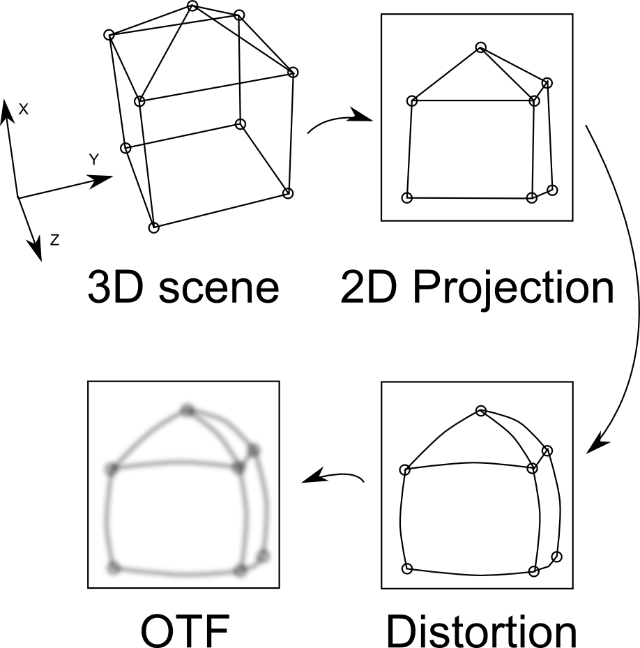
We know at least six 3D points in the scene ($X, Y$ and $Z$ coordinates) and their location at the camera sensor in pixel coordinates. We would like to find the location and orientation of the camera.

Basics

If your object has 6 known points (known 3D coordinates, $X, Y$ and $Z$) you can compute the location of the camera related to the objects coordinate system.

First some basics.

Homogenous coordinate is vector presentation of euclidean coordinate $(X,Y,Z)$ in which we have appended so called scale factor $\omega$ such that the homogenous coordinate is $\textbf{X}=\omega \begin{bmatrix}X & Y & Z & 1\end{bmatrix}^T$. In your own calculations try to keep $\omega=1$ as often as possible (meaning that you “normalize” the homogenous coordinate by dividing it with its last element: $\textbf{X} \leftarrow \frac{\textbf{X}}{\omega}$). We can also use homogenous presentation for 2D points such that $\textbf{x}=\omega\begin{bmatrix}X & Y & 1\end{bmatrix}$ (remeber that these $\omega, X,Y$ and $Z$ are different for each point, be it 2D or 3D point). Homogenous coordinate presentation makes the math easier.

Camera matrix is $3\times4$ projection matrix from the 3D world to the image sensor:

$$
\textbf{x}=P\textbf{X}
$$

Where $\textbf{x}$ is the point on image sensor (with pixels units) and $\textbf{X}$ is the projected 3D point (lets say that it has millimeters as its units).

We remember that cross product between two 3-vectors can be defined as matrix-vector-multiplication such that:

$$
\textbf{v} \times \textbf{u}=\\
( \textbf{v} )_x \textbf{u}=\\
\begin{bmatrix}
0 & -v_3& v_2 \\
v_3 & 0 & -v_1 \\
-v_2 & v_1 & 0
\end{bmatrix}
\textbf{u}
$$

It is also useful to note that cross production $\textbf{v} \times \textbf{v}=\textbf{0}$.

Now lets try to solve the projection matrix $P$ from the previous equations. Lets multiply the projection equation from the left side with $\textbf{x}$s cross product matrix:

$$
(\textbf{x})_x\textbf{x}=(\textbf{x})_xP\textbf{X}=\textbf{0}
$$

Aha! The result must be zero vector. If we now open the equation we get:

$$
\begin{bmatrix}
0 & -w& y \\
w & 0 & -x \\
-y & x & 0
\end{bmatrix}
\begin{bmatrix}
P_{1,1} & P_{1,2} & P_{1,3} & P_{1,4} \\
P_{2,1} & P_{2,2} & P_{2,3} & P_{2,4} \\
P_{3,1} & P_{3,2} & P_{3,3} & P_{3,4}
\end{bmatrix}
\textbf{X}
\\=\begin{bmatrix}
P_{3,4} W y – P_{2,1} X w – P_{2,2} Y w – P_{2,4} W w + P_{3,1} X y – P_{2,3} Z w + P_{3,2} Y y + P_{3,3} Z y \\
P_{1,4} W w + P_{1,1} X w – P_{3,4} W x + P_{1,2} Y w – P_{3,1} X x + P_{1,3} Z w – P_{3,2} Y x – P_{3,3} Z x \\
P_{2,4} W x + P_{2,1} X x – P_{1,4} W y – P_{1,1} X y + P_{2,2} Y x – P_{1,2} Y y + P_{2,3} Z x – P_{1,3} Z y
\end{bmatrix}=\textbf{0}
$$

With little bit of refactoring we can get the projection matrix $P$ outside of the matrix:

$$
\tiny
\begin{bmatrix} 0 & 0 & 0 & 0 & – X\, w & – Y\, w & – Z\, w & – W\, w & X\, y & Y\, y & Z\, y & W\, y\\ X\, w & Y\, w & Z\, w & W\, w & 0 & 0 & 0 & 0 & – X\, x & – Y\, x & – Z\, x & – W\, x\\ – X\, y & – Y\, y & – Z\, y & – W\, y & X\, x & Y\, x & Z\, x & W\, x & 0 & 0 & 0 & 0 \end{bmatrix}
\begin{bmatrix}
\textbf{P}_1 \\
\textbf{P}_2 \\
\textbf{P}_3 \\
\end{bmatrix}=\textbf{0}
$$

Where $\textbf{P}_n$ is the transpose of $n$:th row of the camera matrix $P$. Last row of the previous (big) matrix equation is linear combination of the first two rows, so it does not bring any additional information and it can be left out.

Small pause so we can gather our toughs. Note that the previous matrix equation has to be formed for each known 3D->2D correspondence (there must be at least 6 of them).

Now, for each point correspondence, calculate the first two rows of the matrix above, stack the $2\times12$ matrices on top of each other and you get new matrix $A$ for which

$$
A\begin{bmatrix}
\textbf{P}_1 \\
\textbf{P}_2 \\
\textbf{P}_3 \\
\end{bmatrix}=\textbf{0}
$$

As we have 12 unknowns and (at least) 12 equations this can be solved. Only problem is that we don’t want to have the trivial answer where
$$
\begin{bmatrix}
\textbf{P}_1 \\
\textbf{P}_2 \\
\textbf{P}_3 \\
\end{bmatrix}=\textbf{0}
$$

Fortunately we can use singular value decomposition (SVD) to force

$$
|
\begin{bmatrix}
\textbf{P}_1 \\
\textbf{P}_2 \\
\textbf{P}_3 \\
\end{bmatrix}
|=1
$$

So to solve the the equations, calculate SVD of matrix $A$ and pick the singular vector corresponding to the smallest eigen value. This vector is the null vector of matrix A and also the solution for the camera matrix $P$. Just unstack the $\begin{bmatrix} \textbf{P}_1 & \textbf{P}_2 & \textbf{P}_3 \end{bmatrix}^T$ and form $P$.

Now you wanted to know the distance to the object. $P$ is defined as:

$$
P=K\begin{bmatrix}R & -R\textbf{C}\end{bmatrix}
$$

where $\textbf{C}$ is the camera location relative to the objects origin. It can be solved from the $P$ by calculating $P$s null vector.

Finally, when you calculate the cameras location for two frames, you can calculate the unknown objects locations (or locations of some of the points of the object) by solving two equations for $X$:

$$
\textbf{x}_1=P_1 \textbf{X} \\
\textbf{x}_2=P_2 \textbf{X} \\
$$

Which goes pretty much the same way as how we solved the camera matrices:
$$
(\textbf{x}_1)_xP_1\textbf{X}=\textbf{0} \\
(\textbf{x}_2)_xP_2\textbf{X}=\textbf{0} \\
$$

And so on.


  1. Harley, Zisserman – Multiple View Geometry 2004. Algorithm 7.1 

Camera geometry basics

This article tries to list minimum amount of math which is required for some of the other articles.

Symbols used by this site

  • Scalars are in italics
    • $x$ and $y_0$ are scalars
  • Vectors are bolded
    • $\mathbf{x}$ and $\mathbf{\hat{x}}$ are vectors
  • Matrices are usually upper case letters without italics or bolding
    • $\mathrm{P}$ and $\mathrm{H}$ are matrices

Common symbols

  • $\mathrm{P}$ is $3\times4$ projection matrix
    • $\mathrm{P}=\mathrm{K}[\mathrm{R -R}\mathbf{C}]$
  • $\mathrm{K}$ is $3\times3$ camera calibration matrix
  • $\mathrm{R}$ is $3\times3$ rotation matrix
  • $\mathbf{C}$ is $3\times1$ vector presenting camera center
  • $\mathbf{T}$ is $3\times1$ vector presenting camera translation
    • $\mathbf{T}=-\mathrm{R}\mathbf{C}$
  • $\textbf{x}$ is $3\times1$ homogenous 2D point
  • $\textbf{l}$ is $3\times1$ homogenous 2D line
  • $\textbf{X}$ is $4\times1$ homogenous 3D point
  • $\mathrm{H}$ is $3\times3$ homography/transformation matrix
  • $\omega$ is scalar presenting the “scale” of homogenous coordinate

Vector dot product

Vector dot product is defined for all vectors regardless of the dimension. For two same size vectors, $\mathbf{a}=[a_1, a_2, …, a_n]$ and $\mathbf{b}=[b_1, b_2, …, b_n]$, dot product is defined as $\mathbf{a} \cdot \mathbf{b}=\sum_{i=1}^n a_ib_i$.

Dot product has also geometric interpretation: if the two vectors are interpreted to exist in euclidean space the dot product then relates to cosine of the angle between the two vectors. More specifically $\mathbf{a} \cdot \mathbf{b}=|\mathbf A|\,|\mathbf B|\cos\theta$ where $\theta$ is the angle between the vectors.

This geometric interpretation can be useful for example when similarity between two vectors is compared, if the two vectors point to same direction, angle between the vectors is small and therefore $\cos\theta$ is large. If the angle between the vectors is large $\cos\theta$ is small (or zero if the vectors are prependicular).

(1)

Vector cross product

Vector cross product is defined for two 3-vectors and it produces new vector which is perpendicular to both of the vectors. As now the angle of the new vector is 90° to both original vectors, this means that dot product between the new and old vectors is zero.

Cross product between two 3-vectors, $\mathbf{v}=[v_1, v_2, v_3]$ and $\mathbf{u}=[u_1, u_2, u_3]$, is defined as:
$$
\mathbf{u} \times \mathbf{v}=\begin{bmatrix}
u_2v_3 – u_3v_2 \\
u_3v_1 – u_1v_3 \\
u_1v_2 – u_2v_1 \\
\end{bmatrix}^T
$$
Note that this can also be presented in matrix form:
$$
\mathbf{v} \times \mathbf{u}=[ \mathbf{v} ]_\times \mathbf{u}=\begin{bmatrix}
0 & -v_3& v_2 \\
v_3 & 0 & -v_1 \\
-v_2 & v_1 & 0
\end{bmatrix}
\mathbf{u}
$$

(2, 3)

Homogenous coordinates

Homogenous coordinates are system of coordinates which is commonly used for projective geometry instead of Cartasian coordinates. Instead of using two scalars to present 2D point in homogenous coordinates 2D point is presented using 3 scalars. For example 2D point $\mathbf{x}$ which is in Cartesian coordinates presented as $(x,y)$ is presented in homogenous
coordinates as:
$$
\mathbf{x}=\begin{bmatrix}
\omega x \\
\omega y \\
\omega
\end{bmatrix}=\omega
\begin{bmatrix}
x \\
y \\
1
\end{bmatrix}
$$

Homogenous coordinates are used to present both 2D and 3D points. 3D points are just 4-vectors: $\mathbf{X}=\omega [x,y,z,1]^T$

Why should we use homogenous coordinates?

Homogenous coordinates make it easier to handle projective geometry.

For example lets try to translate non-homogenous 2D point $\mathbf{x_{2d}}=[x,y]^T$ two units to the positive x-direction using matrix multiplication with matrix
$$
\mathrm{H_{2d}}=\begin{bmatrix}
h_{1,1} & h_{1,2} \\
h_{2,1} & h_{2,2}
\end{bmatrix}
$$
$$
\mathbf{x_{translated}}=\mathrm{H_{2d}}\mathbf{x_{2d}}=\begin{bmatrix}
h_{1,1} & h_{1,2} \\
h_{2,1} & h_{2,2}
\end{bmatrix}
\begin{bmatrix}
x \\
y
\end{bmatrix}=\begin{bmatrix}
h_{1,1}x+h_{1,2}y \\
h_{2,1}x+h_{2,2}y \\
\end{bmatrix}
$$
As all elements of $\mathbf{x_{translated}}$ depend on $\mathrm{H_{2d}}$ it is easy to see that 2D translation can not be done with $2\times2$ matrix multiplication.

But if we use homogenous coordinates and $3\times3$ transformation matrix we can define translation as:
$$
\mathrm{H}\mathbf{x}=\begin{bmatrix}
1 & 0 & \delta x \\
0 & 1 & \delta y \\
0 & 0 & 1 \\
\end{bmatrix}
\omega
\begin{bmatrix}
x \\
y \\
1 \\
\end{bmatrix}=\omega
\begin{bmatrix}
x + \delta x \\
y + \delta y \\
1 \\
\end{bmatrix}
$$

If after transformation we get homogenous coordinate for which the $\omega$ is not $1$, we can simply divide the result with $\omega$ and get more easily read presentation of the point/line.

(4, 5)

2D Line

Useful way to define a line is: $\mathbf{l}=[a, b, c]^T$, point $\mathbf{x}$ is on the line if $\mathbf{x} \cdot \mathbf{l}=0$ or $ax + by + c=0$.

If we need to find line $\mathbf{l}$ which travels trough two 2D points, $\mathbf{x_1}$ and $\mathbf{x_2}$, it can be found easily by taking cross product of the two points: $\mathbf{l}=\mathbf{x_1} \times \mathbf{x_2}$. Result can be easily verified if we rember the properties of the cross product and dot product:

  • Cross product results in a vector which is perpendicular to both original vectors.
  • Dot product results is scalar which is directly proportional to the cosine of the angle between the two vectors.
    • If the two orignal vectors are perpendicular the result is 0.

Same way it easy to find point $\mathbf{x}$ in which two lines, $\mathbf{l_1}$ and $\mathbf{l_2}$ cross each other: $\mathbf{x}=\mathbf{l_1} \times \mathbf{l_2}$.

(4)

Links


  1. Wikipedia: Dot product 
  2. Wikipedia: Cross product 
  3. Hartley, Zisserman – Multiple view geometry, 2004. A4.3, p.581. Cross products 
  4. Hartley, Zisserman – Multiple view geometry, 2004. A2.2.1, p.26. Points and lines 
  5. Wikipedia: Homogenous coordinates 

Audible altimeter part 4

After testing the altimeter for about 20-30 jumps I concluded that the short battery life was the most irritating limitation of the altimeter for every day use.

At this stage the MCU was constantly running at 48MHz and display update rate and sensor readings were done at 10/5Hz update rate. The current consumption (without using the beeper) was approximately 27mA@4V which should yild approximately 15 hours of usage with 400mAh battery. Actual usage felt much shorter, maybe only about four or five hours.

Lowest voltage which allows the altimeter to boot up successfully is around 3.0V. First signs of malfunction are the display turning off. With 3.0V battery voltage the current consumption is about 23mA.

The beeper seemed to use additional 100mA (peak).

Current consumption with 24MHz clock, idle

Current consumption ~17mA.

Current consumption with 12MHz clock, idle

Current consumption ~11mA.

Current consumption int main() {}

With default CPU clock. Current consumption ~6mA.

Current consumption with sleep (idle)

~20mA.

Notes

These measurements are made with the first completed altimeter v3.0 which had the MS5805-02BA01 barometer soldered, but not used (measurements not read).

Audible altimeter part 3

The altimeter has been in use for approximately four months and nobody has died. Project is deemed great success and I can finally update the blog.

Actually now the PCB is in version 3 and fourth version is planned. More about progress of the PCB later.

Previous versions

So currently the PCB is at version 3. Version 1 was very quick and rough layout (45mm x 80mm) just to get the project started. It also contained GPS module but the there were lots of mistakes while laying the board near the module and I could not get connection to any satellites. I will be building new PCB for the GPS module again this winter but I’m fairly sure that the GPS can not fit into the existing case as it requires quite large and intact ground plane.

PCB version 1 with GPS and lots of green wire.

Second version was designed around small project case (30mm x 52mm) and contained mounting holes in each corner of the PCB. Micro-USB connector was planted on the long side of the PCB and for testing the buzzer there was two overlapping footprints for different buzzer components.

I ordered small laser cut acrylic case with 1mm wall thickness for the electronics but the case was too flimsy for actual use. The case laser cut profile was designed using MakerCase.

PCB version 2 with acrylic case.

Stencil

Version 3 PCBs arrived after three weeks of waiting.

Version 3 PCBs.

Before starting the altimeter project I had decided to start using reflow soldering. I build small oven controller which uses thermocouple, solid state relay, PWM and PID to control the oven temperature. Stencil for the applying the solder was ordered from OSH Stencils.

Laying components

Most of the components were from Digikey but only place I could find the display was Mouser.

Components.
Major components ready to be placed.
Smaller components were placed first. Most of the resistors and capacitors are 0603 size.
All components laid. Few footprints were left empty as accelerometer and second and third barometer were left out.
Close-up.

Reflow soldering

PCB was reflow soldered in small pizza oven which was connected to temperature controller (visible in the back). Temperature was monitored using terminal application.

Bad component connections

Applying the solder and the whole reflow soldering is not fully in my control as some of the components “tombstoned” (other end of the component lifted from the pad) or solder bridges were formed.

I used head mounted magnifier for inspection. This one has quite poor optical quality and ergonomics.
Bad connection / tombstoning.
Solder bridge under removed capacitor which shorted the 3.3V rail to ground.

Version 3 – Bad traces

After assembling the PCB the USB failed to work. After pullimg my hair for few minutes I noticed that some of the USB traces were missing. This was fixed with small jumper wire.

I contacted OSH Park and let them know about the bad quality just so that process could be improved. They replied quickly and offered refund or free rush order + shipping. Good customer support!

Missing traces.
Good PCB.

First boot

The MCU was programmed using Atmel ICE programmer. I’m using Tag-Connect cables as they have quite small footprint.

Programming.
After few hours of work, it works!

Display connector

As the display connector is only component on the back side of the PCB I soldered it by hand.

Working display. These images are actually from second build which I gave to a friend. The first one I’m using inside the helmet. My friend is using his mostly under canopy as it is wrist mounted.

Case

The PCB was designed to fit into one of the cheap but sturdy plastic cases.
First top of the case was removed.
Then the edges were sanded smooth.
I used two roughness of sandpaper.
Extra parts of version 2 case were used as new top/window.
Holes for the buttons and buzzer.

Cutting holes for the USB and power switch.

Looking “good”. This display is actually LS013B4DN04. LS013B7DH03 is on the right. After a quick test I switched to LS013B7DH03 as I was afraid that the mirror like quality of LS013B4DN04 would not make good contrast in sunny weather.
After some cleanup.
Ready to swoop.

Audible altimeter part 2

Below is notes about the components chosen for the first version of the altimeter and some notes.

  • Air pressure changes approximately 1.44kPa / 100m
  • Sensor interface: i2c
    • SPI would be easier to interface with, but I2C is better learning experience
    • The USB library I’m planning on using has also I2C module (1)
  • MCU: atxmega128a4u
    • 1.6V-3.6V
    • max 32MHZ @ 2.7V
    • max 12MHZ @ 1.6V
    • max 12mA @ 32MHZ @ 3.0V + 0.5mA from 32MHz internal OSC
    • I/O max 20mA per pin
    • 4.5€ @ Digikey
  • Barometer: Freescale: MPL3115A2 (2)
    • Pressure, temperature and altitude
    • 20bit
    • 50kPa – 110kPa (= >4000m – 0m)
    • 0.3m resolution
    • 0.1kPa relative accuracy (changing temperature)
    • Probably not very good for this purpose, but is cheap (2.5€) and gets the project started
    • 6ms-512ms / sample
    • 8.5µA-40µA-265µA@3.3V 1Hz update rate
    • I2C
    • 2.9€ @ Digikey
    • 2V – 3.6V
  • Barometer2: Measurement Specialties: MS5805-02BA01
    • 1.8V – 3.6V
  • Acceleration/heading: InvenSense MPU-9250 (3)
    • Just for the fun of it
    • Barometer data might be little bit boring while developing
    • 5mA max?
    • I2C
    • 11€
    • 2.4V – 3.6V
  • GPS: Linx FM Module
    • http://www.linxtechnologies.com/resources/data-guides/rxm-gps-fm.pdf
    • 3.0V – 4.3V
  • GPS: SIM33ELA ?
  • GPS antenna: Pulse W3011A
  • Hymidity sensor: Silicon Labs 336-2540-1-ND
    • I2C
    • 1.9V – 3.6V
  • Clock: Microchip MCP7940M (4)
    • MCU could do everything this chip can do, but why not just add another i2c chip?
    • 1.2µA@3.3V timekeeping
    • 0.69€ @ Digikey MCP7940MT-I/MNY MCP7940MT-I/MNYCT-ND
    • I2C
    • 1.8V – 5.5V
  • Crystal Oscillator
    • 0805
    • 0.9€ @ Digikey CM315D32768EZFT 300-8816-1-ND
    • +-20ppm
  • Display: LS013B4DN04 / LS013B7DH03
    • 32mm x 28mm x ~1.5mm
    • 2.7V – 3.3V
    • 12µW dynamic display @ 1Hz
    • 15€ (Mouser)
  • FPS connector
    • SFV10R-2STE1HLF 609-4306-1-ND – Top contacts
    • SFV10R-1STE1HLF 609-4305-1-ND – Bottom contacts <- Use this for 180 bent (under PCB)
    • 0.55€ (Digikey)
    • 0.5mm pitch
    • 0.3mm FPC thickness
    • 0.7€ @ Digikey
  • Buzzer
    • CSS-0575A-SMT-TR 102-2201-1-ND
    • 3.7€ (Digikey)
    • 5mm x 5mm x 2.4mm
    • Drive with NPN BJT + 180 OHM + protective diode
    • 3.2€ @ Digikey
    • 2V – 4V
  • USB charging IC
    • MCP73831 http://www.digikey.fi/product-detail/en/MCP73831T-2ACI%2FOT/MCP73831T-2ACI%2FOTCT-ND/1979802
    • Sparkfun
    • 0.4€ @ Digikey
  • USB connector
    • Micro B
    • 0.4€ @ Digikey 609-4616-1-ND or 609-4618-1-ND
  • Micro SD card slot
    • 1.1€ @ Digikey 101-00660-68-6-1-ND
  • Flash memory
    • S25FL216K
    • 2.7V – 3.6V
    • SOIC-8
  • 3.3V supply IC
    • Linear regulator
    • Reasoning: For 3.3V linear offers ~90% efficiency. 2.7V design would not benefit much more. Switching regulator would require board space and add complexity. Maybe next time.
    • Reasonable transient characteristics? (AND9089-D)
    • 0.7€ @ Digikey NCP4681DSQ33T1G NCP4681DSQ33T1GOSTR-ND
  • 400mAh battery: 403035
    • 35mm x 30mm x 4mm
    • 7€ (ebay)
    • 3.7V
    • 2.7V – 4.5V
  • Current consumption active:
    • 13mA: MCU
    • 0.3mA: Barometer
    • 5mA: 9Axis
    • 0.001mA: Clock
    • 0.015mA: Display
    • <= 20mA (buzzer not included)
    • = 20h @ 400mAh
  • Current consumption waiting:
    • 1mA: MCU (MAX) (active 1MHz)
    • 0.01mA: Barometer
    • 0.015mA: Display
    • <= 2mA
    • >= 1 week
  • For 9 month battery life
    • 400mAh / 24309h = 62µA
    • 5µA: MCU (32kHZ)
    • ~1µA LDO
    • 1.2µA: Clock
    • = Should be possible

Links

Audible altimeter part 1

Intro

As the skydiving season in Finland is nearing its end it is time to find something elso to do at weekends. As I just got the A-license I have been gathering necessary equipment for the sport. Only the audible altimeter is missing as I can not decide between Altimaster N3 and L&B Protrack (1, 2).

I have always had problems to finish electronics projects and I think that it might be related to the fact that the end result of the project would have not seen any actual use. By creating something which is useful at one of my hobbies I hope that I have enough motivation to finish the project.

Audible altimeters are used to alert skydivers with loud alarm when they pass certain altides in freefall or with the canopy. In Finland the audible altimeter can only be used as a secondary altimeter as some kind of visual (digital or analog display) altimeter is required by the regulations. As I’m going to be carrying a visual altimeter I feel it will be relatively safe to test my own electronic projects while skydiving.

I’m using Cookie G3 (3) which has two small pockets (~5cm x ~5cm) for audibles. If the electronics catches on fire I plan on installing simple cutaway system (4) for the helmet .

Even if the project fails, I hope it will create good material for some other website (5, 6).

Requirements

  • Approximate size: 5cm x 5cm x 1cm
    • Neptune N3: 6.2cm x 4.3cm x 1.2cm
    • Optima II: 5.6cm x 4.1cm x 1.1cm
    • 5cm x 3.2cm x 1.6cm fits Cookie G3 nicely
    • Current PCB 50mm x 35mm
  • USB rechargeable battery
  • Audible alarm
  • Relatively good altitude accuracy (+-50m) with small lag
  • Simple logging capability

Advanced options

  • Accelerometer/attitude
  • GPS
  • Simple display
  • Led indicator for the alarms as in Optima 2 (7)

Links

Wingsuit part 1

Few years ago I saw video (1) of a home build mianiature parachute made by my friend Tuukka. The video inspired me quite a bit as before the video I didn’t feel like you could actually build any real “hardware” for skydiving without going to rigging courses and practicing a lot. I felt that designing and building parachute would be too much for my skills, but maybe I could still make something from fabrics.

In 2017 Tuukka jumped his home build and desinged parachute (2).

At the end of 2016 skydiving season I borrowed a sewing machine, purchaced cheap fabric and spend one evening sewing my very first tracking pants without any sewing patterns. The pants were huge failure (air intakes tore and the pants functioned as a air brakes), but hey, at least I created something.

During the winter I designed first tracking pants which I tested on the first jump of 2017. Unfortunately the design was not very good and the crotch seam and fabric was torn after two jumps while squatting on the ground.

Next there was a design for tracking jacket, but the design for the shoulders was so bad that I didn’t jump any jumps with the thing.

Finally third tracking pants+jacket design was relative good and I was able to have glide ratio around 1.1.

Natural progress towards diy wingsuit required diy one-piece tracking suit so I build one in late 2017. The suit was little bit hard to fly and I’m still not sure of performance of the suit. But at least it looked quite nice.

In December 2017 I started designing the diy wingsuit. I looked at beginner/advanced beginner level wingsuits from different manufacturers and draw a outline of the wingsuit in Inkscape. I used my friends Colugo 2 wingsuit to get idea of the details. Design was done once again in Clo3d/Clo. It took approximately 10-15 hours to design the suit. I ordered the pattern from a printing company which specializes in construction design drawings. This way I didn’t have to tape more than a hundred A4s together to get the full pattern.

Cutting the patterns took only about one hour. Cutting and sewing the first arm wing took about 9 hours, with the second one I made few stupid mistakes and had to unpick the half finished wing back to its basic components.

Quite soon I realized that the leg wing had a design flaw as it did not extend over the buttocks as all commercial wingsuits. Unfortunately at this point modifications were too hard to make for my skills, but I decided to complete the suit.

After about total of 60-120 hours of work the suit was finished. The arm wings still were little bit rough as the sewing machine started to malfuncion at the very last hours.

Finally in 2018-04-22 I did first jump with the wingsuit (also my very first wingsuit jump). The suit was very stable and the jump went well. In 2018 I had about 6 jumps with the wingsuit, every one of them quite stable (except when trying backflying). I can achieve around 1.8 glide ratio (wind compensated) with the suit, but I think the GL could be much better with practice.

Unfortunately when moving away from Finland, I had to leave the suit to storage as space in the van was very limited.

Hopefully I return to the suit at some point, maybe I will get few jumps with ‘real’ suits in between.

Links

Missing TensorRT documentation for createNMSPlugin layer

Update: Some of TensorRT plugins were released as open source. Old version of NMS is located at https://github.com/NVIDIA/TensorRT/tree/master/plugin/nmsPlugin and new version can be found at https://github.com/NVIDIA/TensorRT/tree/master/plugin/batchedNMSPlugin .

While trying to convert Tensorflow detection network to TensorRT I needed to either implement new non-maximum suppression layer or to use NVIDIAs createNMSPlugin layer. After quick look trough the poor documentation (1, 2) I was forced to just experiment with the layer by feeding it different size inputs and hoping to get it working.

After few hours of frustrating trial and error experimentation I implemented new NMS plugin layer using 3. Unfortunately this implementation did not have very good performance which I think is because of synchronization operations used in 3. 4 would probably have been better alternative as it is lower level and leaves synchronization for the developer.

Fortunately with help of coworkers we were finally able figure out proper inputs for the plugin. Hopefully this helps some one else.

Inputs

  • Prediction locations from the network. Shape of the tensor needs to be [4*number_of_boxes, 1, 1]. Or [4*number_of_boxes*number_of_classes, 1, 1] if shareLocation parameter is set to true in DetectionOutputParameters.
  • Class confidence tensor. Shape [number_of_classes*number_of_boxes, 1, 1]
  • Prior box locations and variances. Shape [2, number_of_boxes*4, 1].

You can change the input order by setting inputOrder parameter in DetectionOutputParameters.

Outputs

  • Final prediction boxes. Shape [1, keep_topk, 7]. [ImageId, Label, Confidence, Xmin, Ymin, Xmax, Ymax]
  • Number of valid boxes [1,1,1]. This value is int32.

Input format of tensors

Prior box locations and variances must have format:

[[box1_prior1, box1_prior2, box1_prior3, box1_prior4]
[box2_prior1, box2_prior2, box2_prior3, box2_prior4]
...
[box1_variance1, box1_variance2, box1_variance3, box1_variance4]
[box2_variance1, box2_variance2, box2_variance3, box2_variance4]
...]

The box format can be chosen using codeType in DetectionOutputParameters.